Sector 6 by default displays a spectrogram of the dynamics of RR intervals for the entire study period (Fig. 2.20). A spectrogram is a graphical representation of the performed spectral analysis of a sequence of RR intervals. If you look at the CIG (Fig. 2.18), you can see that the RR-interval values fluctuate, and the CIG itself consists of both fast and slow oscillations. Spectral analysis makes it possible to identify which frequencies make the greatest contribution to the pattern of the cardiointervalogram. All possible frequencies (see the horizontal scale in Fig. 2.20) fit in the range from 0 to 0,5 Hertz (Hz). Classically, the following are distinguished: the very low frequency range, or VLF (up to 0,04 Hz), the low frequency range, or LF (from 0,04 Hz to 0,15 Hz), and the high frequency range, or HF (above 0,15 Hz). Spectral analysis is most informative when the duration of the ECG recording in a certain stationary state is 5 minutes or more.
Under the conditions of testing in Stressonika, the recordings are short. Therefore, only the low-frequency (LF) and high-frequency (HF) ranges and their ratio are digitized in sector 6 (Fig. 2.20).
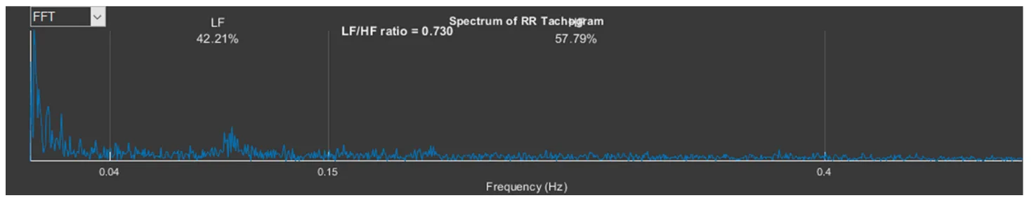
Figure 2.21. Spectrogram of the dynamics of RR intervals for the “BreathOE” stage
We remind you that work with sector 6 is related to work in sector 1; for example, activating the “BreathOE” stage in sector 1 will lead to recalculation of the spectrogram only for this stage (Fig. 2.3). Let us consider the resulting spectrogram more closely (Fig. 2.21).
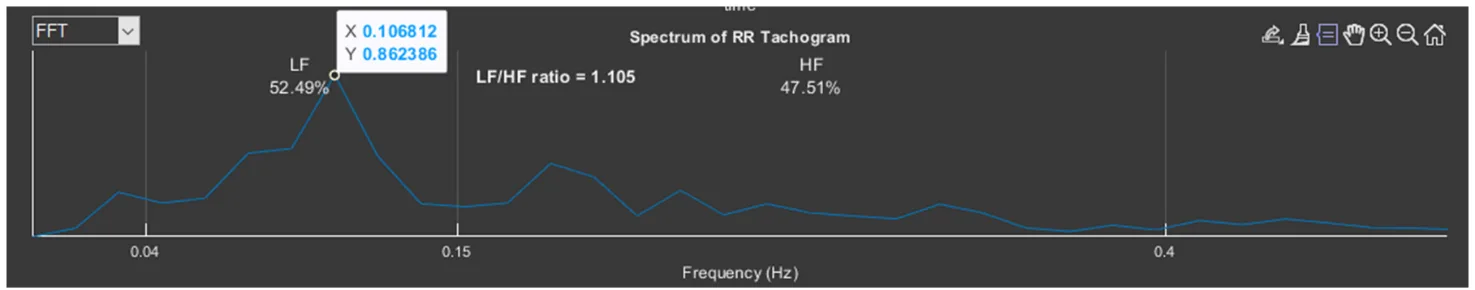
Figure 2.21. Spectrogram of the dynamics of RR intervals for the “BreathOE” stage
We draw attention to the fact that the spectrogram shows a slight dominance of the low-frequency range (52,49%), which was also reflected in the LF/HF ratio (it is greater than 1). Using “Data Tips”, let us mark the peak on the spectrogram: frequency – 0,107 Hz (or 6,4 per min); amplitude – 0,862 ms2. And now let us look at Fig. 2.19a. This is what the sequence of RR intervals looks like, on the basis of which this spectrogram was built. As we remember, this is related to the task of slow (6 breathing movements per minute), rhythmic, imposed breathing with open eyes. Ideal performance of this test would appear in the form of a high-amplitude sinusoid-like CIG curve with 6 waves. The CIG graph presented in Fig. 2.19a resembles such a curve only very remotely, which is confirmed by spectral analysis: a moderate predominance of LF, the frequency characteristic of the peak on the spectrogram differs somewhat from the frequency of the imposed rhythm (0,1 Hz), and the peak amplitude is less than 1.
This example is also only for becoming acquainted with the “Cardio domain” page. We will consider details and specifics in the next chapter.
In the upper left corner of sector 6 there is a window that allows the spectrogram to be replaced with an angle histogram on the scatter plot located in sector 7. To do this, it is necessary to activate the list for selecting the image in sector 6: FFT (Fast Fourier transform) – to select the spectrogram; “angles” – to select the angle histogram (Fig. 2.22a). By default, a spectrogram is displayed in the sector; if we select “angles”, an histogram is displayed (Fig. 2.22b). The step of our histogram is 10°, and the height of a bar is the number of angles that were recorded in this range (Fig. 2.22c: range 20-30° – 1 angle, 80-90° – 9). The histogram clearly shows which angles were more frequent at the stage activated in sector 1 (Fig. 2.3b). In Fig. 2.22b it is clearly visible that during the “BreathOE” stage there were more angles exceeding 90°. It is considered that when the sympathetic nervous system is activated, the histogram density shifts to the left, i.e., toward acute angles.
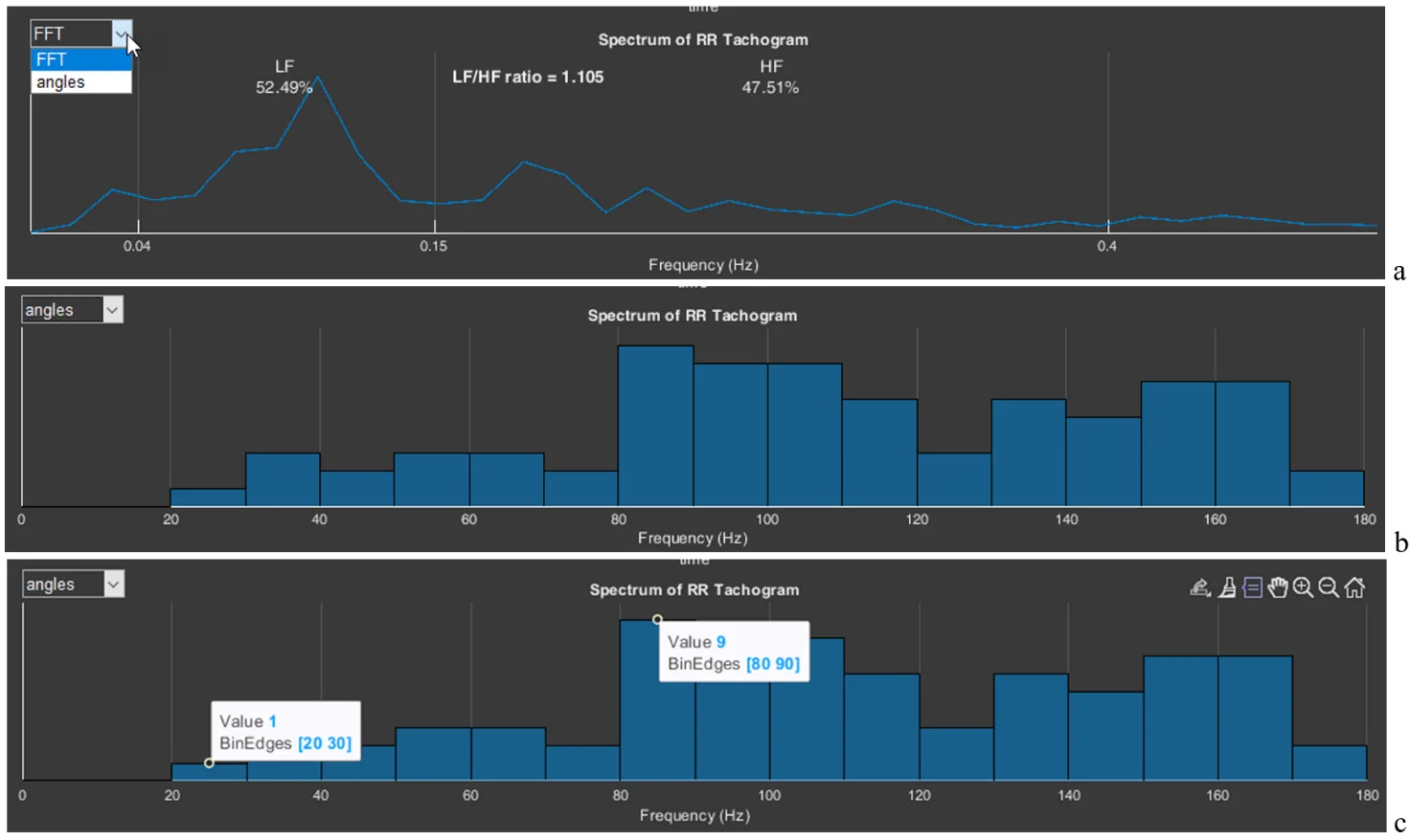
Figure 2.22. Stages of switching from a spectrogram to an angle histogram on the scatter plot (explanations in the text).
This HRV assessment approach is one of the geometric methods.