4.4.1. Fourier (STFT — Short-Time Fourier Transform) #
Method: Spectrogram using windowed FFT.
Parameters:
- Window: Hamming
- Window length:
window = Fs * window_length_seconds - Overlap:
nooverlap = window - 25
(to ensure smoothness)
Formula:[S, F, T, P] = spectrogram(signal, hamming(window), nooverlap, window, Fs, 'power', 'yaxis')
Display:
- X-axis: time
- Y-axis: frequency (0–50 Hz)
- Color: logarithmic power (10*log10(P))
- Color range: -15 to 25 dB
Interpretation: Shows how signal power is distributed across frequencies over time. Brighter colors = higher power.
How to read a spectrogram:
- Horizontal axis (X): recording time
- Vertical axis (Y): frequency (0–50 Hz)
- Color: power (brighter = more power)
Typical patterns:
- Horizontal bands: stable rhythms
- a band at 10 Hz = alpha rhythm (relaxation)
- a band at 20 Hz = beta rhythm (activity)
- Vertical bands: short events
- blink artifacts (low frequencies, short duration)
- muscle artifacts (high frequencies, short duration)
- Changes over time: state transitions
- alpha to beta when opening the eyes
- beta to alpha when closing the eyes
Physiological interpretation:
A spectrogram is a “map” of brain activity over time and frequency. It shows which frequency components are present at each moment.
- Bright band in the alpha range (8–13 Hz): relaxed state, eyes closed
- Bright band in the beta range (13–30 Hz): active thinking, concentration
- Low power across all ranges: possible artifacts or pathology
- Sharp changes: state transitions, responses to stimuli
4.4.2. Wavelet #
Method: Wavelet Packet Decomposition.
Parameters:
- Decomposition level: 8
- Wavelet type: selected from the list (for example, db4, coif2, sym4)
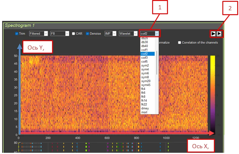
- 1. Wavelet type: select from the drop-down list
- 2. Data recalculation buttons
Formula:wpt = wpdec(signal, 8, wavelet_type)
[P, T, F] = wpspectrum(wpt, Fs)
P = flipud(P)
Interpretation: Similar to STFT, but with better time resolution at high frequencies and better frequency resolution at low frequencies.
Advantages for EEG:
- High frequencies (beta, gamma): short windows make it possible to determine the exact event time
- Low frequencies (alpha, theta): long windows provide better frequency resolution
Physiological meaning:
Wavelet transformation uses windows of variable length—short windows for high frequencies and long windows for low frequencies. This corresponds well to the way the brain processes information.
- Fast processes (for example, a response to a stimulus) require precise time resolution.
- Slow rhythms (for example, alpha) require precise frequency resolution.
- Wavelet transformation provides an optimal balance.
When to use:
- For analyzing rapid events (responses to stimuli)
- For analyzing slow rhythms with high precision
- When both time and frequency resolution are needed simultaneously
4.4.3. Hilbert (Hilbert–Huang Transform) #
Method: Hilbert–Huang Transform using EMD.
Parameters:
- Frequency resolution: 1 Hz
Formula:[P, F, T] = hht(signal, Fs, 'FrequencyResolution', 1)
Interpretation: Adaptive decomposition into intrinsic modes followed by analysis of instantaneous frequency. Suitable for nonlinear and non-stationary signals.
Physiological explanation of HHT:
The Hilbert–Huang Transform combines EMD (decomposition into modes) with instantaneous frequency analysis. This makes it possible to track how the frequency of a rhythm changes over time.
Physiological meaning:
- The alpha rhythm frequency is not constant; it may “drift” from 8 to 13 Hz.
- HHT shows these changes in instantaneous frequency.
- This is important for understanding rhythm dynamics.
Advantages:
- Adaptivity: adjusts to the signal
- Nonlinearity: can process nonlinear phenomena
- Instantaneous frequency: shows frequency changes over time
When to use:
- For analyzing non-stationary signals (whose properties change over time)
- For tracking rhythm frequency drift
- For analyzing complex nonlinear processes